大家好,今天和各位分享一下如何使用 TensorFlow 构建 ViT B-16 模型。为了方便大家理解,代码使用函数方法。
1. 引言
在计算机视觉任务中,注意力机制通常被用来增强特征或替换一些卷积层来优化网络结构。这些方法利用注意力机制来增强原有卷积网络结构中的特征。
[En]
In computer vision tasks, attention mechanism is usually used to enhance features or to replace some convolution layers to optimize the network structure. * these methods use attention mechanism to enhance features in the original convolution network structure.*
而 ViT 依赖于原有的编码器结构进行搭建,并将其用于图像分类任务,在减少模型参数量的同时提高了检测准确度。
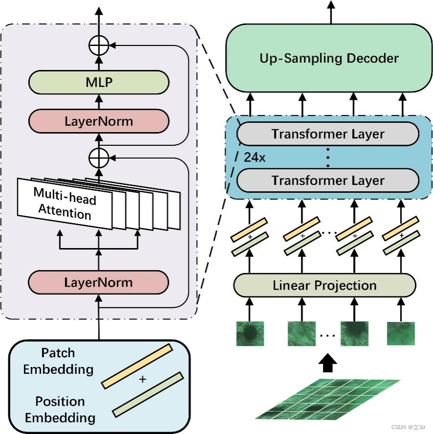
将 Transformer 用于图像分类任务主要有以下 5 个过程: (1)将输入图像或特征进行序列化; (2)添加位置编码; (3)添加可学习的嵌入向量; (4)输入到编码器中进行编码; (5)将输出的可学习嵌入向量用于分类。结构图如下:
2. Patch Embedding
import tensorflow as tf
from tensorflow import keras
from tensorflow.keras import layers
以 b2242243 的输入图片为例。首先进行图像分块, 将原图片切分为 1414 个图像块(Patch),每个 Patch 的大小为 1616,*通过提取输入图片中的平坦像素向量,将每个输入 Patch 送入线性投影层,得到 Patch Embeddings。
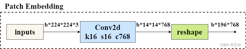
在代码中, 先经过一个 kernel=(16,16),strides=16 的卷积层划分图像块,再将 h和w 维度整合为 num_patches 维度,代表 一共有 196 个 patch,每个 patch 为 16*16
# --------------------------------------------- #
# (1)Embedding 层
# inputs代表输入图像,shape为224*224*3
# out_channel代表该模块的输出通道数,即第一个卷积层输出通道数=768
# patch_size代表卷积核在图像上每16*16个区域卷积得出一个值
# --------------------------------------------- #
def patch_embed(inputs, out_channel, patch_size=16):

    # 获得输入图像的shape=[b,224,224,3]
    b, h, w, c = inputs.shape

    # 获得划分后每张图像的size=(14,14)
    grid_h, grid_w = h//patch_size, w//patch_size

    # 计算图像宽高共有多少个像素点 n = h*w
    num_patches = grid_h * grid_w

    # 卷积 [b,224,224,3]==>[b,14,14,768]
    x = layers.Conv2D(filters=out_channel, kernel_size=(16,16), strides=16, padding='same')(inputs)

    # 维度调整 [b,h,w,c]==>[b,n,c]
    # [b,14,14,768]==>[b,196,768]
    x = tf.reshape(x, shape=[b, num_patches, out_channel])

    return x
3. 添加类别标签和位置编码
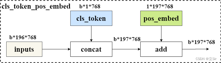
为了输出融合了全局语义信息的向量表示, 在第一个输入向量前添加可学习分类变量。经过编码器编码后, 在最后一层输出中,该位置对应的输出向量就可以用于分类任务。与其他位置对应的输出向量相比, 该向量可以更好的融合图像中各个图像块之间的依赖关系。
在 Transformer 更新的过程中, 输入序列的顺序信息会丢失。Transformer 本身并没有办法学习这个信息,所以 需要一种方法将位置表示聚合到模型的输入嵌入中。我们 对每个 Patch 进行位置编码, 该位置编码采用随机初始化,之后参与模型训练。与传统三角函数的位置编码方法不同, 该方法是可学习的。
最后,将 Patch-Embeddings 和 class-token 进行堆叠,和 Position-Embeddings 进行叠加,得到最终嵌入向量,该向量输入给 Transformer 层进行后续处理。
代码如下:
# --------------------------------------------- #
# (2)类别标签和位置编码
# --------------------------------------------- #
def class_pos_add(inputs):

    # 获得输入特征图的shape=[b,196,768]
    b, num_patches, channel = inputs.shape

    # 类别信息 [1,1,768]
    # 直接通过classtoken来判断类别,classtoken能够学到其他token中的分类相关的信息
    cls_token = layers.Layer().add_weight(name='classtoken', shape=[1,1,channel], dtype=tf.float32,
                                          initializer=keras.initializers.Zeros(), trainable=True)

    # 可学习的位置变量 [1,197,768], 初始化为0,trainable=True代表可以通过反向传播更新权重
    pos_embed = layers.Layer().add_weight(name='posembed', shape=[1,num_patches+1,channel], dtype=tf.float32,
                                          initializer=keras.initializers.RandomNormal(stddev=0.02), trainable=True)

    # 将类别信息在维度上广播 [1,1,768]==>[b,1,768]
    cls_token = tf.broadcast_to(cls_token, shape=[b, 1, channel])

    # 在num_patches维度上堆叠,注意要把cls_token放前面
    # [b,1,768]+[b,196,768]==>[b,197,768]
    x = layers.concatenate([cls_token, inputs], axis=1)

    # 将位置信息叠加上去
    x = tf.add(x, pos_embed)

    return x  # [b,197,768]
4. 多头自注意力模块
Transformer 层中,主要包含多头注意力机制和多层感知机模块,下面先介绍多头自注意力模块。
单个的注意力机制,其每个输入包含三个不同的向量,分别为 Query向量(Q),Key向量(K),Value向量(V)。他们的结果分别 由输入特征图和三个权重做矩阵乘法得到。
接着为每一个输入计算一个得分
为了使梯度稳定, 对 Score 的值进行归一化处理,并 将结果通过 softmax 函数进行映射。之后 再和 v 做矩阵相乘,得到加权后每个输入向量的得分 v。计算完后 再乘以一个权重张量 W 提取特征。
计算公式如下,其中 代表 K 向量维度的平方根
代码如下:
# --------------------------------------------- #
# (3)多头自注意力模块
# inputs: 代表编码后的特征图
# num_heads: 代表多头注意力中heads个数
# qkv_bias: 计算qkv是否使用偏置
# atten_drop_rate, proj_drop_rate:代表两个全连接层后面的dropout层
# --------------------------------------------- #
def attention(inputs, num_heads, qkv_bias=False, atten_drop_rate=0., proj_drop_rate=0.):

    # 获取输入特征图的shape=[b,197,768]
    b, num_patches, channel = inputs.shape
    # 计算每个head的通道数
    head_channel = channel // num_heads
    # 公式的分母,根号d
    scale = head_channel ** 0.5

    # 经过一个全连接层计算qkv [b,197,768]==>[b,197,768*3]
    qkv = layers.Dense(channel*3, use_bias=qkv_bias)(inputs)
    # 调整维度 [b,197,768*3]==>[b,197,3,num_heads,c//num_heads]
    qkv = tf.reshape(qkv, shape=[b, num_patches, 3, num_heads, channel//num_heads])
    # 维度重排 [b,197,3,num_heads,c//num_heads]==>[3,b,num_heads,197,c//num_heads]
    qkv = tf.transpose(qkv, perm=[2, 0, 3, 1, 4])
    # 获取q、k、v的值==>[b,num_heads,197,c//num_heads]
    q, k, v = qkv[0], qkv[1], qkv[2]

    # 矩阵乘法, q 乘 k 的转置,除以缩放因子。矩阵相乘计算最后两个维度
    # [b,num_heads,197,c//num_heads] * [b,num_heads,c//num_heads,197] ==> [b,num_heads,197,197]
    atten = tf.matmul(a=q, b=k, transpose_b=True) / scale
    # 对每张特征图进行softmax函数
    atten = tf.nn.softmax(atten, axis=-1)
    # 经过dropout层
    atten = layers.Dropout(rate=atten_drop_rate)(atten)
    # 再进行矩阵相乘==>[b,num_heads,197,c//num_heads]
    atten = tf.matmul(a=atten, b=v)

    # 维度重排==>[b,197,num_heads,c//num_heads]
    x = tf.transpose(atten, perm=[0, 2, 1, 3])
    # 维度调整==>[b,197,c]==[b,197,768]
    x = tf.reshape(x, shape=[b, num_patches, channel])

    # 调整之后再经过一个全连接层提取特征==>[b,197,768]
    x = layers.Dense(channel)(x)
    # 经过dropout
    x = layers.Dropout(rate=proj_drop_rate)(x)

    return x
5. MLP 多层感知器
这部分简单的由两个完全连通的层来提取特征,流程图如下。第一全连接层通道增加4倍,第二全连接层通道减少到原来的水平。
[En]
This part is simply two fully connected layers to extract features, the flow chart is as follows. The first full connection layer channel increases 4 times, and the second full connection layer channel decreases to the original.
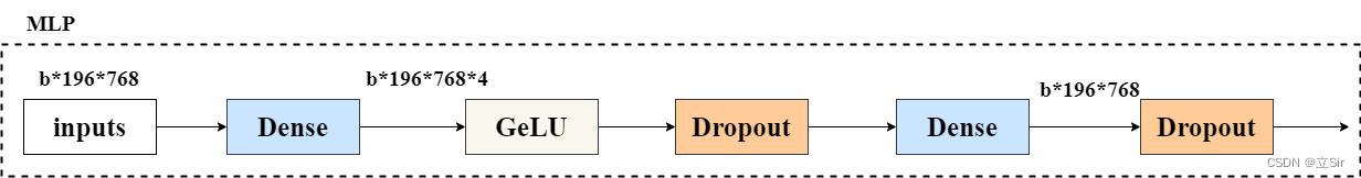
代码如下:
# ------------------------------------------------------ #
# (4)MLP block
# inputs代表输入特征图;mlp_ratio代表第一个全连接层上升通道倍数;
# drop_rate代表杀死神经元概率
# ------------------------------------------------------ #
def mlp_block(inputs, mlp_ratio=4.0, drop_rate=0.):

    # 获取输入图像的shape=[b,197,768]
    b, num_patches, channel = inputs.shape

    # 第一个全连接上升通道数==>[b,197,768*4]
    x = layers.Dense(int(channel*mlp_ratio))(inputs)
    # GeLU激活函数
    x = layers.Activation('gelu')(x)
    # dropout层
    x = layers.Dropout(rate=drop_rate)(x)

    # 第二个全连接层恢复通道数==>[b,197,768]
    x = layers.Dense(channel)(x)
    # dropout层
    x = layers.Dropout(rate=drop_rate)(x)

    return x
6. 特征提取模块
Transformer 的 单个特征提取模块是由 多头注意力机制和 多层感知机模块组合而成,encoder_block 模块的流程图如下。
输入图像像经过 LayerNormalization 标准化后,再经过我们上面定义的多头注意力模块,将输出结果和输入特征图残差连接, 图像在特征提取过程中shape保持不变。
然后对输出进行标准化,然后送到多层感知器提取特征,然后用残差连接输入和输出。
[En]
The output is then standardized, and then sent to the multi-layer perceptron to extract features, and then the residual is used to connect the input and output.
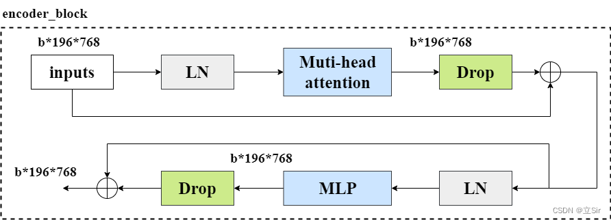
而 transformer 的特征提取模块是由多个 encoder_block 叠加而成, 这里连续使用12个 encoder_block 模块来提取特征。
代码如下:
# ------------------------------------------------------ #
# (5)单个特征提取模块
# num_heads:代表自注意力的heads个数
# epsilon:小浮点数添加到方差中以避免除以零
# drop_rate:自注意力模块之后的dropout概率
# ------------------------------------------------------ #
def encoder_block(inputs, num_heads, epsilon=1e-6, drop_rate=0.):

    # LayerNormalization
    x = layers.LayerNormalization(epsilon=epsilon)(inputs)
    # 自注意力模块
    x = attention(x, num_heads=num_heads)
    # dropout层
    x = layers.Dropout(rate=drop_rate)(x)
    # 残差连接输入和输出
    # x1 = x + inputs
    x1 = layers.add([x, inputs])

    # LayerNormalization
    x = layers.LayerNormalization(epsilon=epsilon)(x1)
    # MLP模块
    x = mlp_block(x)
    # dropout层
    x = layers.Dropout(rate=drop_rate)(x)
    # 残差连接
    # x2 = x + x1
    x2 = layers.add([x, x1])

    return x2  # [b,197,768]

# ------------------------------------------------------ #
# (6)连续12个特征提取模块
# ------------------------------------------------------ #
def transformer_block(x, num_heads):

    # 重复堆叠12次
    for _ in range(12):
        # 本次的特征提取块的输出是下一次的输入
        x = encoder_block(x, num_heads=num_heads)

    return x  # 返回特征提取12次后的特征图
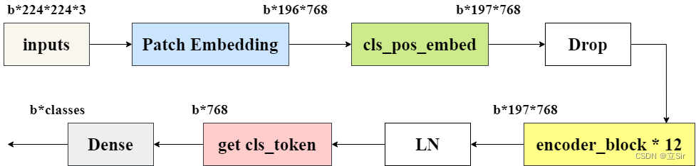
7. 主干网络
接下来,设置网络并将上述所有模块组合在一起,如下图所示。
[En]
Next, set up the network and combine all the above modules together, as shown in the following figure.
在下面代码中要注意的是 cls_ticks = x[:,0]取出所有的类别标签。 因为 在 cls_pos_embed 模块中,我们 将 cls_token 和输入图像在 patch 维度上堆叠 layers.concate,用于学习每张特征图的类别信息,取出的 类别标签 cls_ticks 的 shape 为 [b, 768]。最后经过一个全连接层得出每张图片属于每个类别的得分。
代码如下:
# ---------------------------------------------------------- #
# (7)主干网络
# batch_shape:代表输入图像的shape=[8,224,224,3]
# classes:代表最终的分类数
# drop_rate:代表位置编码后的dropout层的drop率
# num_heads:代表自注意力机制的heads个数
# epsilon:小浮点数添加到方差中以避免除以零
# ---------------------------------------------------------- #
def VIT(batch_shape, classes, drop_rate=0., num_heads=12, epsilon=1e-6):

    # 构造输入层 [b,224,224,3]
    inputs = keras.Input(batch_shape=batch_shape)

    # PatchEmbedding层==>[b,196,768]
    x = patch_embed(inputs, out_channel=768)

    # 类别和位置编码==>[b,197,768]
    x = class_pos_add(x)

    # dropout层
    x = layers.Dropout(rate=drop_rate)(x)

    # 经过12次特征提取==>[b,197,768]
    x = transformer_block(x, num_heads=num_heads)

    # LayerNormalization
    x = layers.LayerNormalization(epsilon=epsilon)(x)

    # 取出特征图的类别标签,在第(2)步中我们把类别标签放在了最前面
    cls_ticks = x[:,0]
    # 全连接层分类
    outputs = layers.Dense(classes)(cls_ticks)

    # 构建模型
    model = keras.Model(inputs, outputs)

    return model
8. 查看模型结构
这里有个注意点, keras.Input() 的参数问题,创建输入层时,参数 shape 不需要指定batch维度,batch_shape 需要指定batch维度。
keras.Input(shape=None, batch_shape=None, name=None, dtype=K.floatx(), sparse=False, tensor=None)
'''
shape: 形状元组(整型),不包括batch size。for instance, shape=(32,) 表示了预期的输入将是一批32维的向量。
batch_shape: 形状元组(整型),包括了batch size。for instance, batch_shape=(10,32)表示了预期的输入将是10个32维向量的批次。
'''
接收模型后,通过 model.summary() 查看模型结构和参数量,通过 get_flops() 参看浮点计算量。
# ---------------------------------------------------------- #
# (8)接收模型
# ---------------------------------------------------------- #
if __name__ == '__main__':

    batch_shape = [8,224,224,3]  # 输入图像的尺寸
    classes = 1000  # 分类数

    # 接收模型
    model = VIT(batch_shape, classes)

    # 查看模型结构
    model.summary()

    # 查看浮点计算量 flops = 51955425272
    from keras_flops import get_flops
    print('flops:', get_flops(model, batch_size=8))
参数量和计算量如下
> Original: https://blog.csdn.net/dgvv4/article/details/124792386
> Author: 立Sir
> Title: 【神经网络】(21) Vision Transformer 代码复现,网络解析,附TensorFlow完整代码
---
---
## **相关阅读**
## Title: Linux服务器成功安装TensorFlow-GPU并成功调用GPU
在我们做深度学习的时候,需要高速大量的运算,这就对我们的设备要求较高。在服务器上运行代码就成了一个不错的选择,但是服务器与我们常用的Windows系统是不一样的,Windows系统是图形交互界面的,我们完成所有的工作只需要点点点就行了,但是服务器就不一样,服务器多数都是命令交互式的,我们需要输入一个命令,然后在去查看或者修改东西。
下面就是在服务器运行深度学习代码的一个基础环境搭建教程,基于TensorFlow的。
假设我们有一台安装了操作系统的全新服务器,那么我们需要采取几个步骤:<details><summary>*<font color='gray'>[En]</font>*</summary>*<font color='gray'>Suppose we get a brand new server with the operating system installed, then we need to take a few steps:</font>*</details>
# 1.重装操作系统(可选):
[重装centos系统教程https://blog.csdn.net/qq_51570094/article/details/124133324 ;](https://blog.csdn.net/qq_51570094/article/details/124133324 "重装centos系统教程")
# 2.安装显卡驱动(可选):
[显卡驱动安装教程https://blog.csdn.net/qq_51570094/article/details/123900837 ;](https://blog.csdn.net/qq_51570094/article/details/123900837 "显卡驱动安装教程")
# 3.安装anaconda3(可选):
[anaconda3安装教程https://blog.csdn.net/qq_51570094/article/details/123903593 ;](https://blog.csdn.net/qq_51570094/article/details/123903593 "anaconda3安装教程")
# 4.安装GUDA和cudnn(可选):
[CUDA 和cudnn安装教程https://blog.csdn.net/qq_51570094/article/details/123902419 ;](https://blog.csdn.net/qq_51570094/article/details/123902419 "CUDA 和cudnn安装教程")
# 5.安装TensorFlow-GPU:
今天我们着重讲解一下如何安装TensorFlow-GPU。
假设我们已将安装好了上面的基础环境,并进行验证。
查看显卡驱动是否安装成功:
nvidia-smi
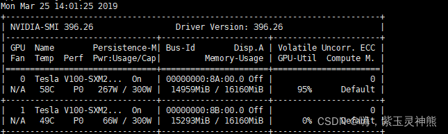
有输出信息则说明显卡驱动安装成功。
查看anaconda3是否安装成功:
conda -V
输出conda的版本信息:

或者查看conda下安装了些什么包:
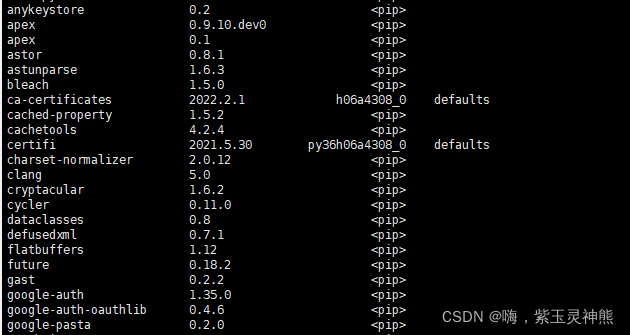
conda list
有输出信息也说明anaconda3安装成功。
查看cuda和cudnn是否安装成功:

可以看到cuda的安装版本是9.2.
下面开始安装TensorFlow-GPU
conda创建一个虚拟环境:
conda create -n tf python=3.6
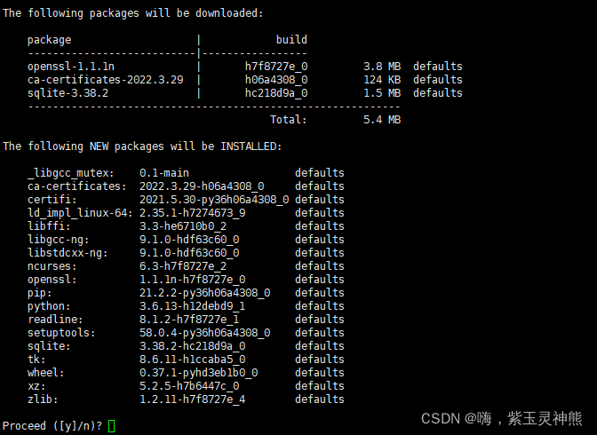
输入y,等待安装完成。
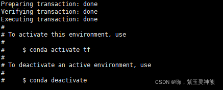
安装完成,激活环境:
conda activate tf
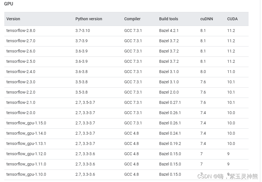
查看各TensorFlow-GPU版本与CUDA,cudnn版本的对应关系,选择合适的版本进行安装:
[TensorFlow-GPU https://tensorflow.google.cn/install/source_windows?hl=en#gpu ;](https://tensorflow.google.cn/install/source_windows?hl=en#gpu "TensorFlow-GPU")
安装TensorFlow-GPU版本,用conda安装:
conda install tensorflow-gpu==1.12.0
也可使用pip安装:调用的是国内镜像豆瓣源,后面的信息表示信任该网站。
pip install tensorflow-gpu==1.12.0 -i http://pypi.douban.com/simple --trusted-host pypi.douban.com
等待安装完成:

验证是否安装成功:
import tensorflow as tf
tf.test.is_gpu_available()
输出如下:
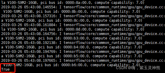
安装成功,并且可以调用GPU。
> Original: https://blog.csdn.net/qq_51570094/article/details/124106174
> Author: 嗨,紫玉灵神熊
> Title: Linux服务器成功安装TensorFlow-GPU并成功调用GPU
> Original: https://blog.csdn.net/dgvv4/article/details/124792386
> Author: 立Sir
> Title: 【神经网络】(21) Vision Transformer 代码复现,网络解析,附TensorFlow完整代码
---
---
## **相关阅读**
## Title: 用Anaconda安装TensorFlow(Windows10)
## 用Anaconda安装TensorFlow
**本部分分为方法一和方法二,方法一是从清华镜像官网下载速度较快,<br> 方法二是从GitHub下载,速度较慢(有梯子的建议使用)**
**1.打开Anaconda Prompt**
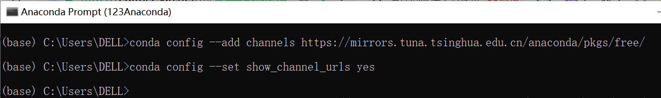
**2.输入下面两行命令,打开清华镜像官网**
```js
conda config --add channels https://mirrors.tuna.tsinghua.edu.cn/anaconda/pkgs/free/
conda config --set show_channel_urls yes
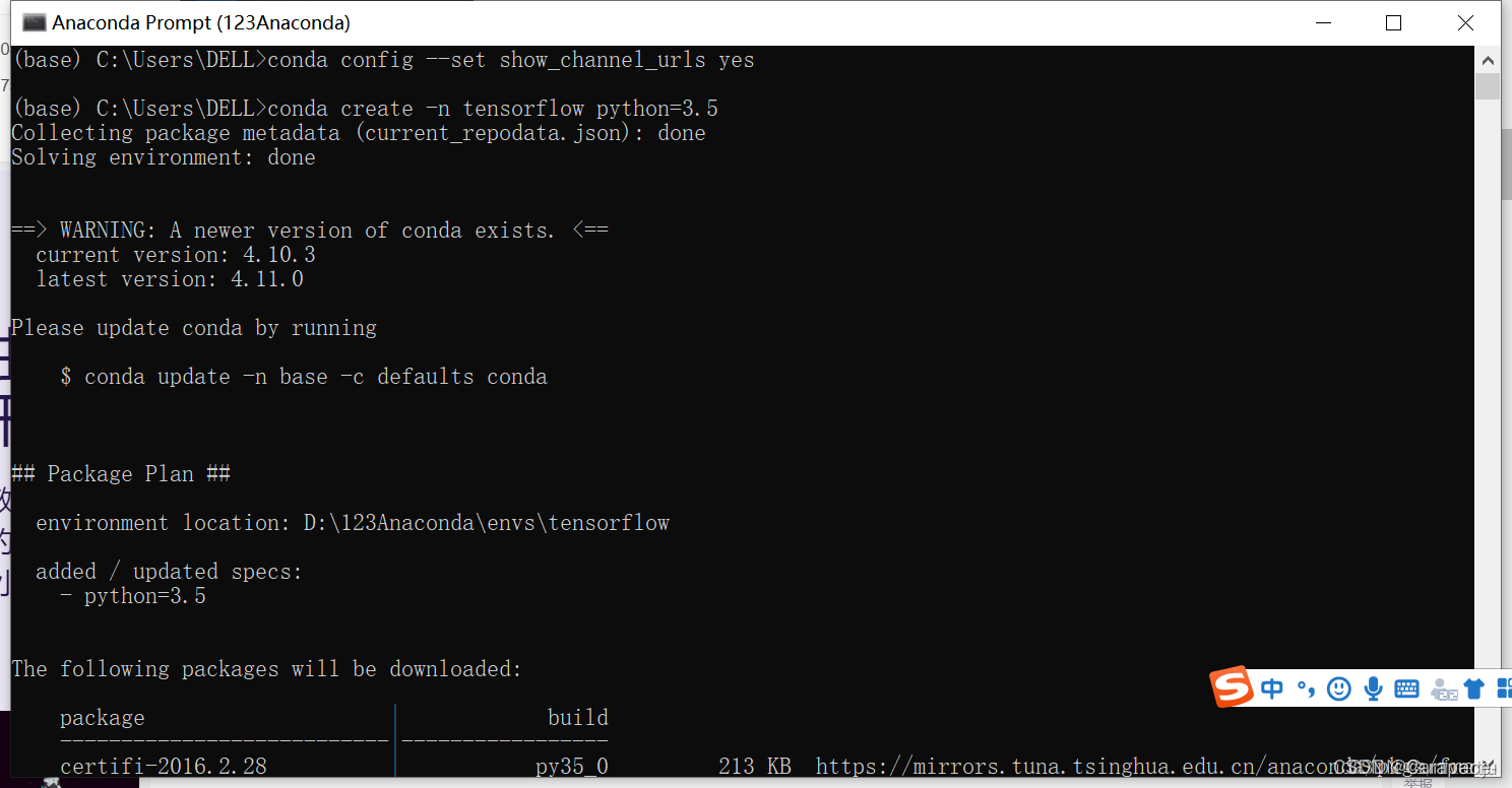
3.输入下面命令,利用Anaconda创建一个python3.9的环境,环境名称为tensorflow(这里python版本根据自己的情况如下图)
conda create -n tensorflow python=3.9
如图所示:
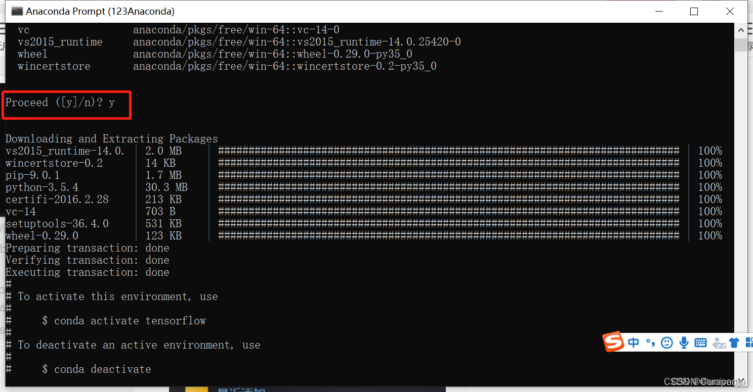
4.输入y
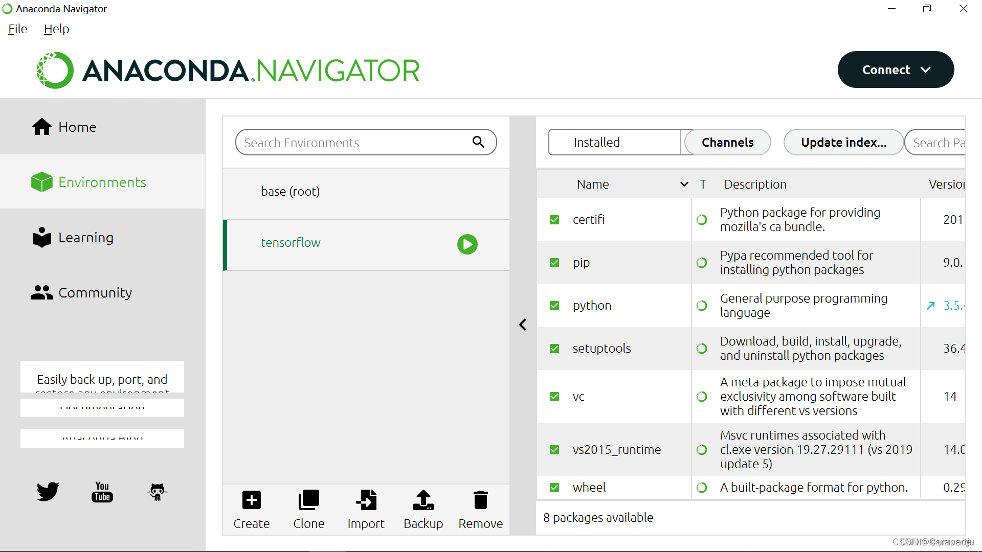
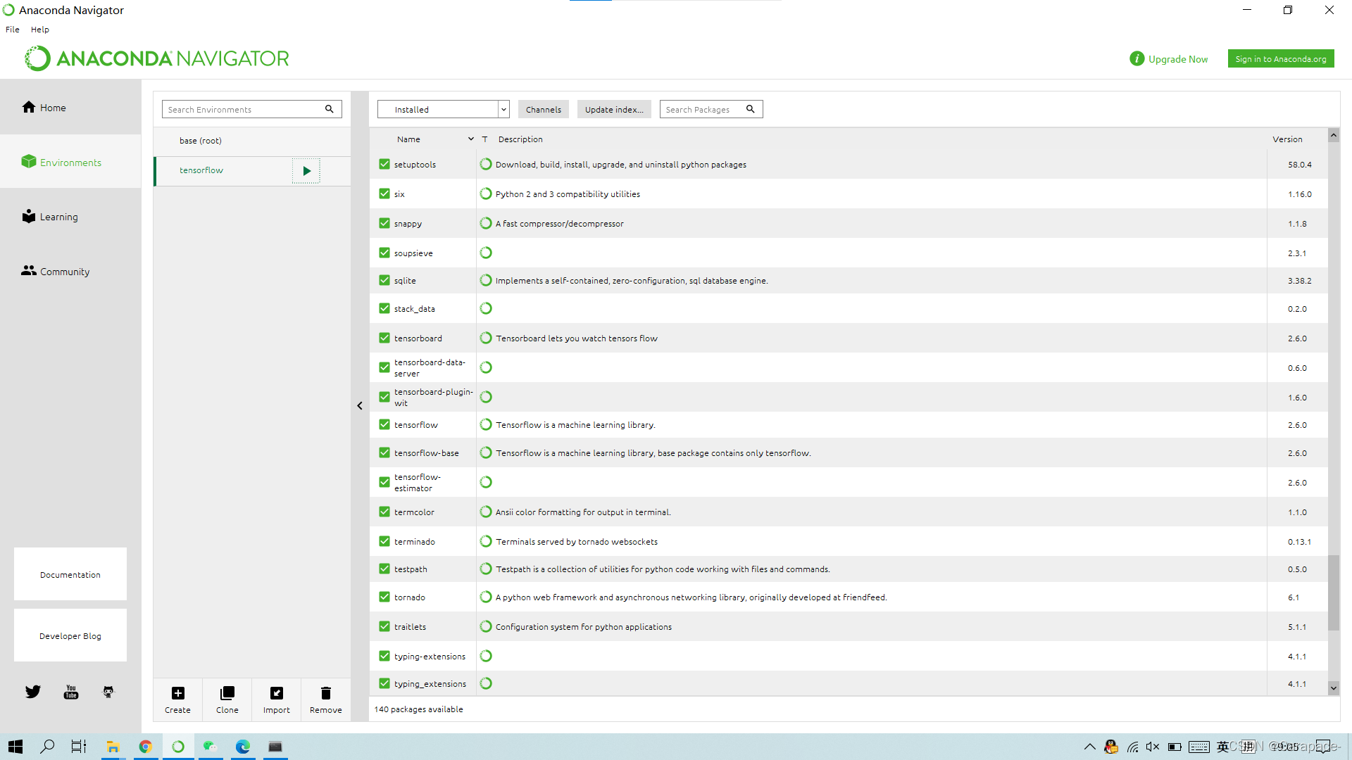
5.打开Anaconda Navigator,点击Environments,可以看到名称为tensorflow的环境已经创建好

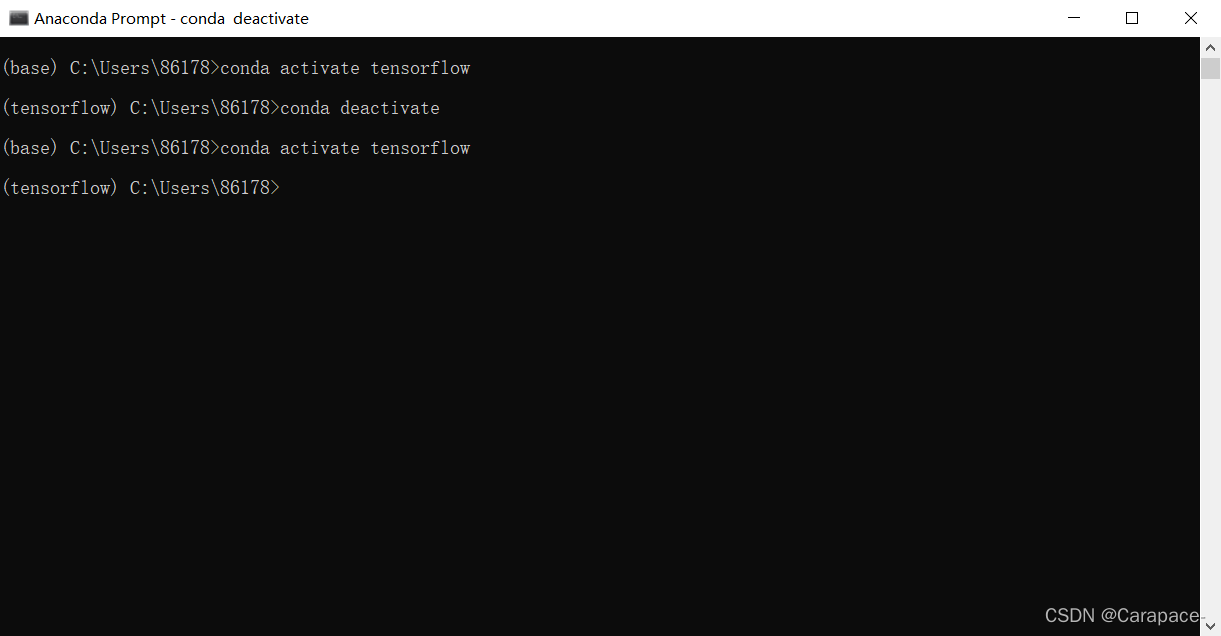
6.上一步最后我们可以看到,启动Tensorflow,使用下面的命令行:
conda activate tensorflow

关闭tensorflow环境,使用下面的命令行:
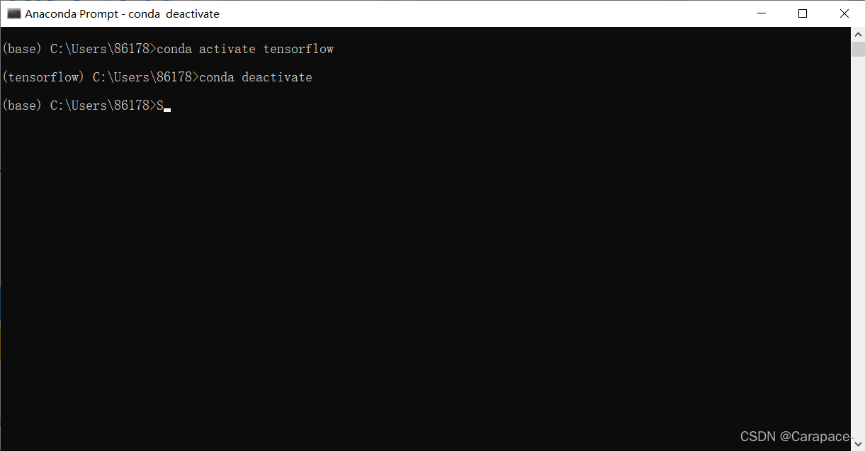
7.我们在这里输入下面的命令,进入tensorflow环境
conda activate tensorflow
8.输入下面的命令行,安装cpu版本的tensorflow
conda install tensorflow
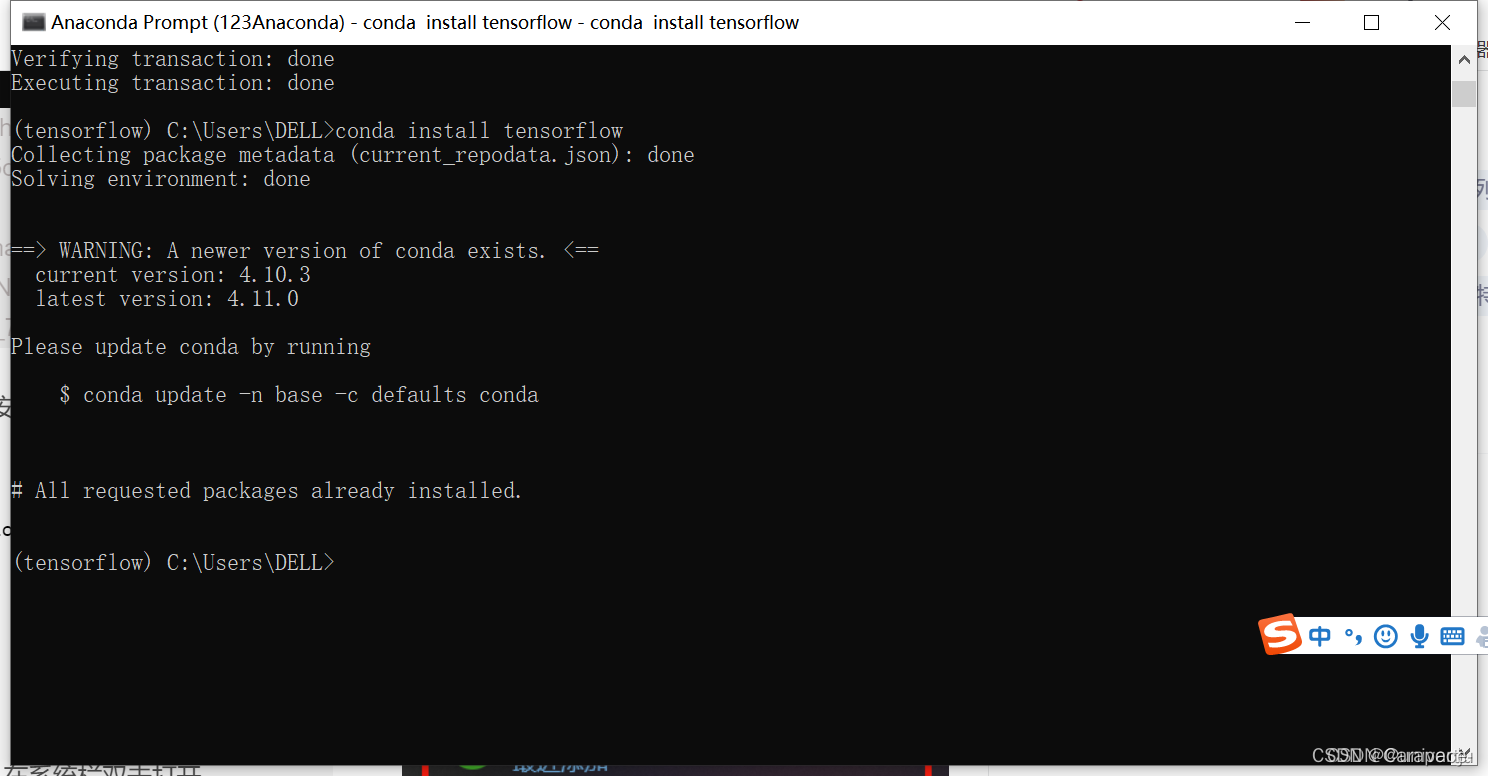
此时我们再次查看Anaconda Navigator中的Environments,可以发现tensorflow已经安装好了
第8步注意!!!
如果出现下图情况或者是从GitHub上下载速度极慢,说明清华镜像网址没有切换成功
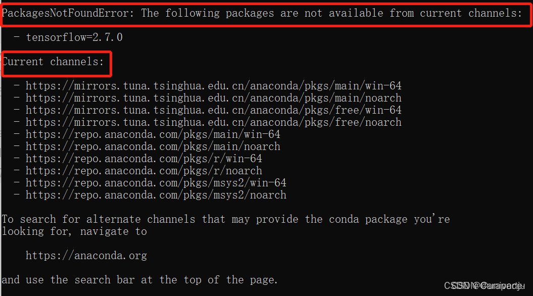
重新执行步骤二即可
TensorFlow安装方法方法二
方法二速度特别特别慢 (如果有梯子的话建议使用)
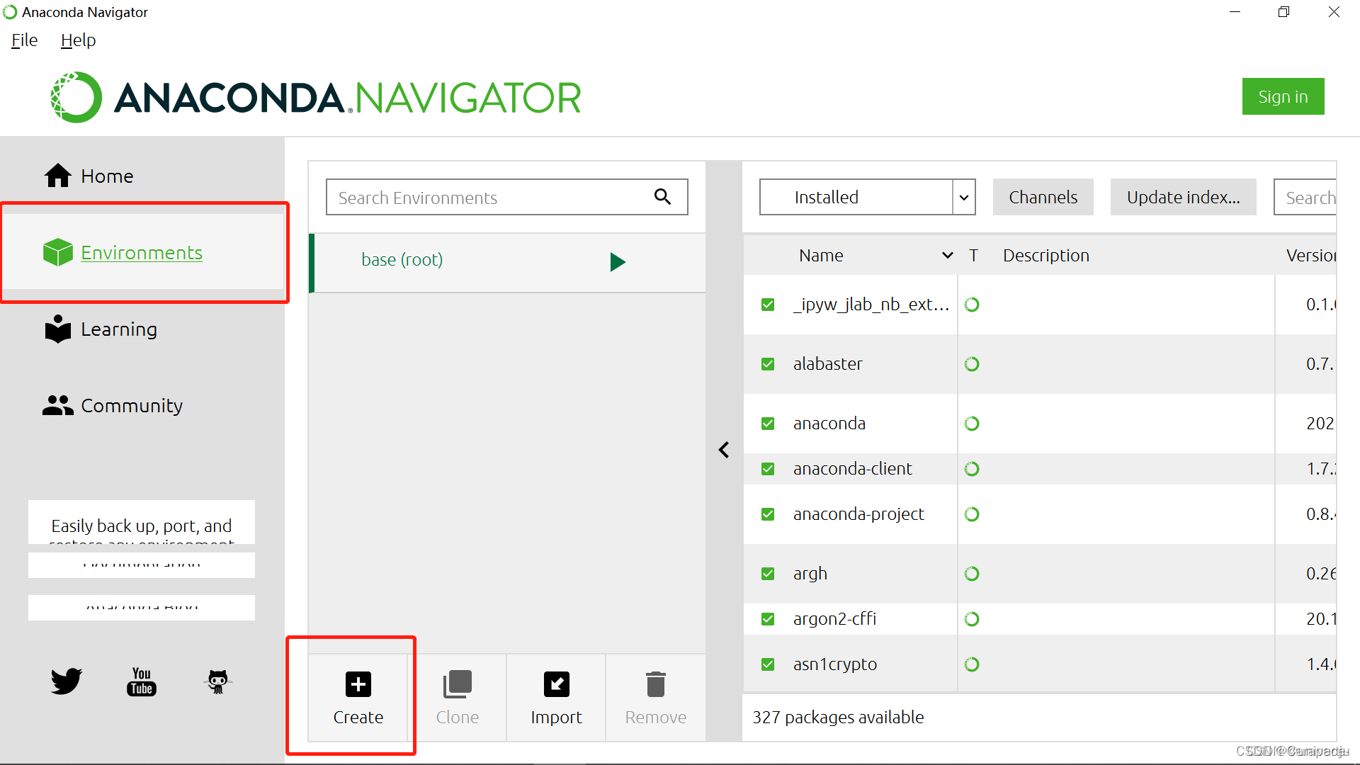
1.安装好Anaconda后,在系统栏双击打开Anaconda Navigator

2.点击Environment,Create
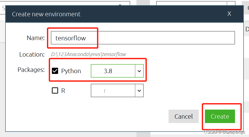
3.创建一个tensorflow的新环境,python在这里可以自行选择(根据Anaconda中安装的python版本,我这里是python3.8),然后点击Create
4.右边搜索栏输入tensorflow,选择后点击Apply
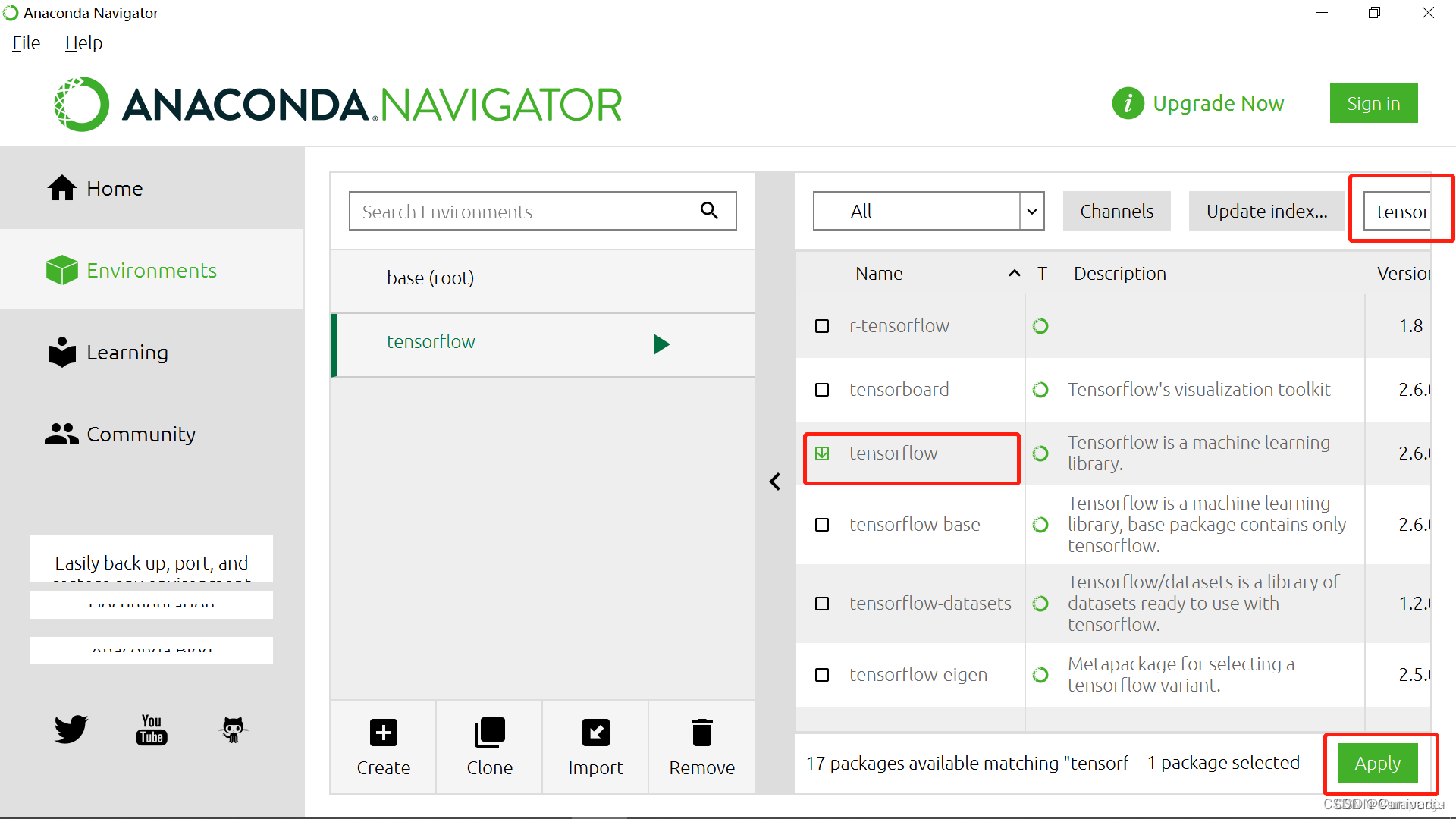
5.点击Apply
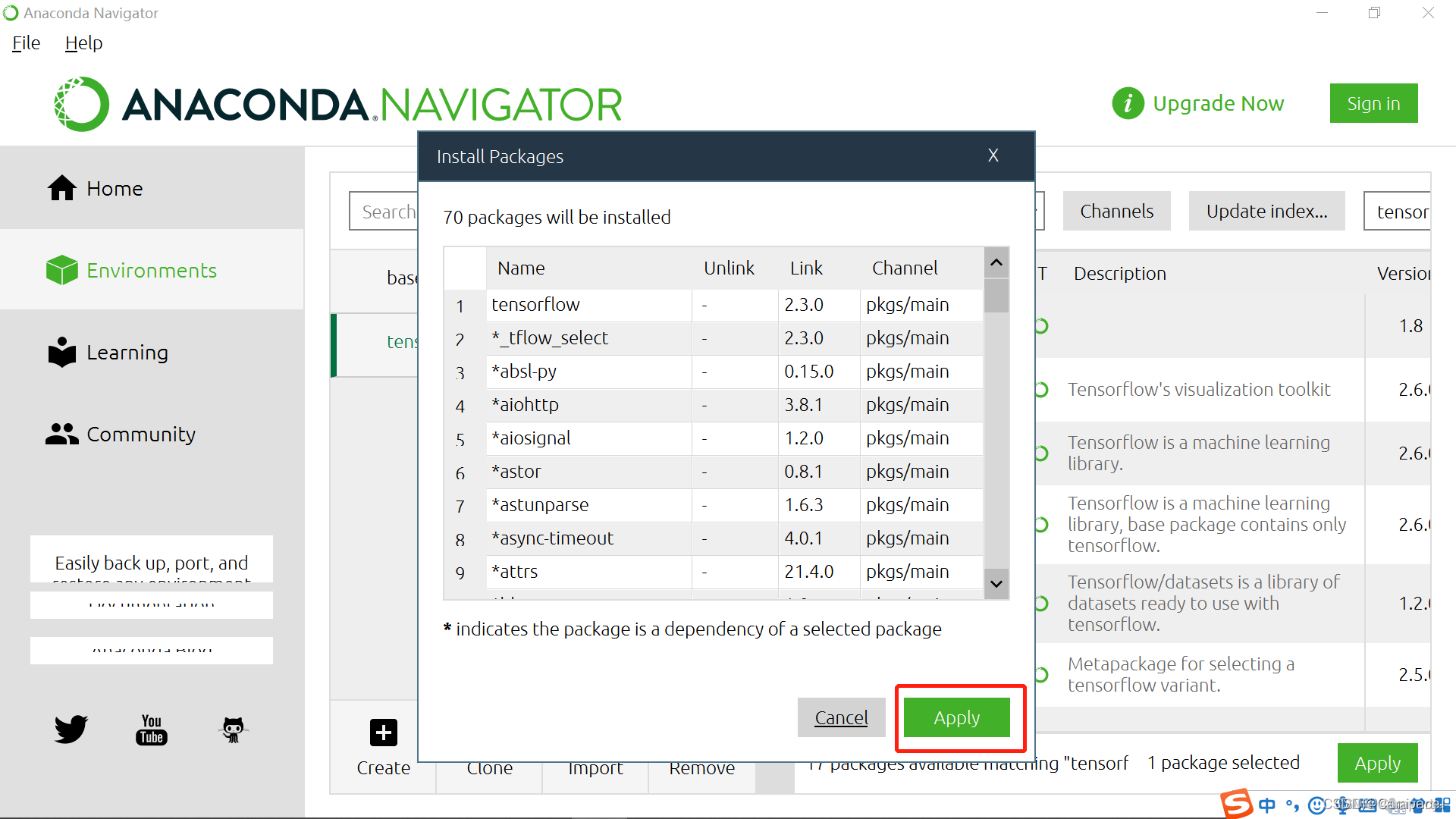
等待安装完成即可
Original: https://blog.csdn.net/m0_46299185/article/details/124280787
Author: bEstow--
Title: 用Anaconda安装TensorFlow(Windows10)