Titanic数据分析

背景

题目参见：Titanic
实际就是根据乘客的性别、年龄、舱位等级等信息预测乘客的成活率。很多人也说这个数据集比较小，使用一些tricky的技术提高准群率意义不大，但是作为练手的项目还是很好的。帮助理解各种数据预处理方法、分类模型还是很有帮助的。

分析和处理

1. 纯Naive的做法：不管三七二十一，输出Survived=0或者1.这当然是一种做法，但是基本没啥意义，但是可以作为之后分类器准确率的参照；
2. 对数据稍作分析：

df = pd.read_csv('train.csv')
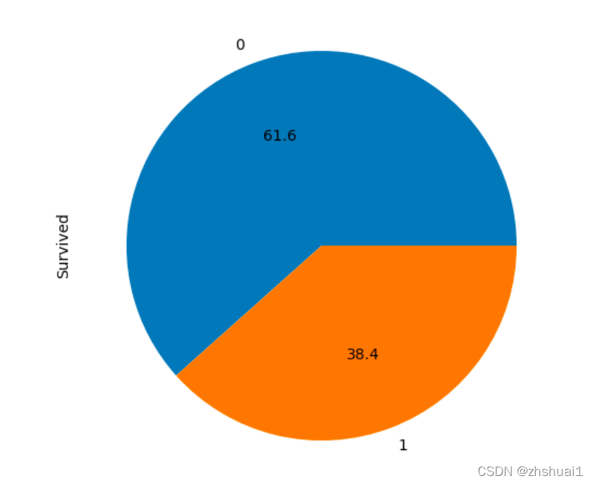
dd = df.groupby('Survived')['Survived'].count()
print(dd.head())
dd.plot(kind='pie', autopct='%1.1f')
plt.show()

从饼状图上看，幸存的人数仍然很少，这实际上可以预测测试集上左右两名乘客的死亡情况，这样正确率可以达到50%以上。当然，这种做法还是没有任何意义，但我们被给予了最低基准，准确率不能低于61%，否则模型肯定有问题，最好不要使用模型。

3. 那我们分各个维度来看看有没有明显的差异。
3.1 性别

df = pd.read_csv('train.csv')
df = df.groupby('Survived')
df0 = df.get_group(0).groupby('Sex')['Sex'].count()
df1 = df.get_group(1).groupby('Sex')['Sex'].count()
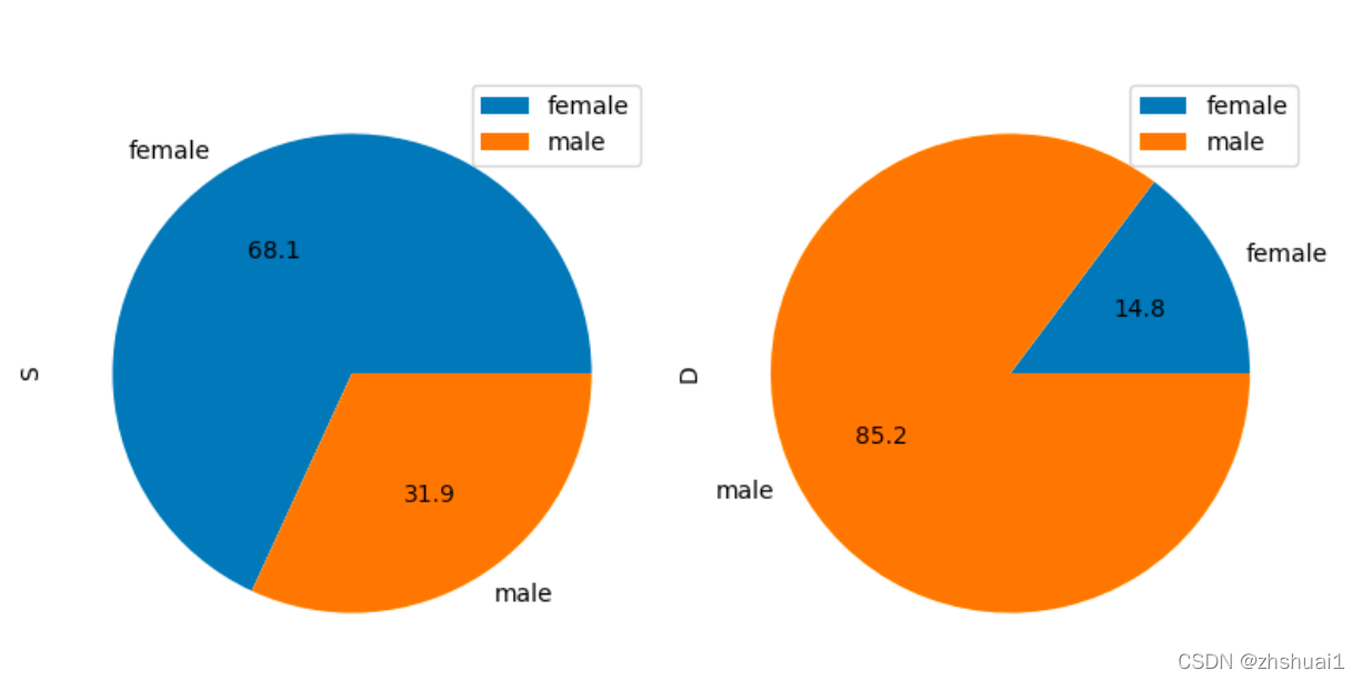
df = pd.DataFrame({"S": df1, "D": df0})
df.plot(kind='pie', autopct='%1.1f', subplots=True, figsize=(8, 8))
plt.show()

可见大部分男性都死亡了，大部分女性都存活了。

使用pivot_table看看

df = pd.read_csv('train.csv')
dd = pd.pivot_table(df, index=['Sex'], columns=['Survived'], values=['Pclass'], aggfunc=[len])
print(dd)

在jupyter里看起来是这样的：

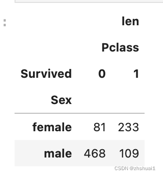
加入我们，简单地说，所有的男人都死了，所有的女人都活着，可以达到预期的争夺率。

233 + 468 81 + 233 + 468 + 109 = 78.6 % \frac {233+468} {81+233+468+109} = 78.6\%8 1 +2 3 3 +4 6 8 +1 0 9 2 3 3 +4 6 8 ​=7 8 .6 %
使用这种方式提交，我们确实可以得到一个比较高的正确率，数据证明可以达到76.55%。所以如果一个模型的正确率连76.55%都打不到，那数据的处理一定是有问题，要么就是模型学习不充分或者过拟合，要么就是特征处理有问题。
3.2 年龄
年龄的处理比较特别：

• 年龄有177字段是缺失的
• 年龄有些小数的数值
• 因为年龄跨度大，但是样本比较少，某些年龄数据可能会很稀疏

对于缺失字段，我们可以1. drop缺失字段；2. 使用缺省值、特殊值进行填充(比如-1或者0等)；3. 使用均值或者众数或者分组众数进行填充；
对于2和3，我们可以使用类似方法进行处理：对不同的年龄进行分组(分桶)。分桶的方式有：1. 区间段分组；2. 哈希分组。相邻的年龄具有相关性，当然使用哈希分组更合理。
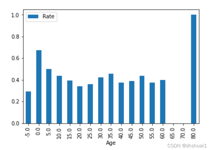
在处理丢失的数据时，我们可能会产生更多有用的信息，或者我们可能会丢失信息。事实上，在分析数据之前，我们还不知道结论。因此，在分析中，我们首先处理的是年龄是否缺失。为了简化处理过程，我们将年龄划分为5岁为间隔，遗漏任务为-5岁作为特殊处理。

df = pd.read_csv('models/titanic/train.csv')
df.loc[df.Age.isnull(),'Age']=-5
df.Age = df.Age // 5 * 5
dd = df.pivot_table(index=['Age'], columns = ['Survived'], values=['PassengerId'],aggfunc=[len]).copy()
dd['Win'] = np.where(dd[('len', 'PassengerId', 0)]>dd[('len', 'PassengerId', 1)],dd[('len', 'PassengerId', 0)],dd[('len', 'PassengerId', 1)])
dd['Win'].sum()/891

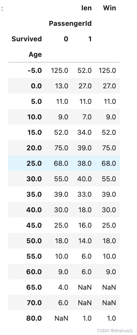
如果按照年龄来推断是否存活，则胜率可以得到62%(其实并不高)
各个年龄段的分布如下

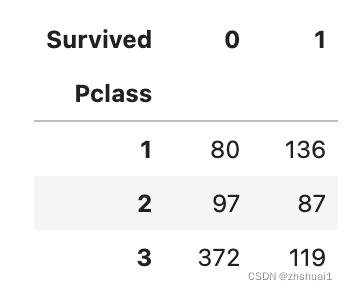
3.3 舱位

df = pd.read_csv('models/titanic/train.csv')
df.pivot_table(index=['Pclass'], columns = ['Survived'], values=['PassengerId'],aggfunc=[len])

诚然，不同客舱的乘客存活率差异很大，但如果仅利用客舱信息进行预测，准确率可达67%，仅略高于完全存活或完全死亡。

这里就有两个问题了：

1. 如何更快的定位哪个特征最重要？(pandas 相关性分析、决策树的顶层节点)
2. 组合特征是否能取得更好的效果？
   我们把舱位和性别两个特征结合起来看

df = pd.read_csv('models/titanic/train.csv')
df.pivot_table(index=['Pclass','Sex'], columns = ['Survived'], values=['PassengerId'],aggfunc=[len])

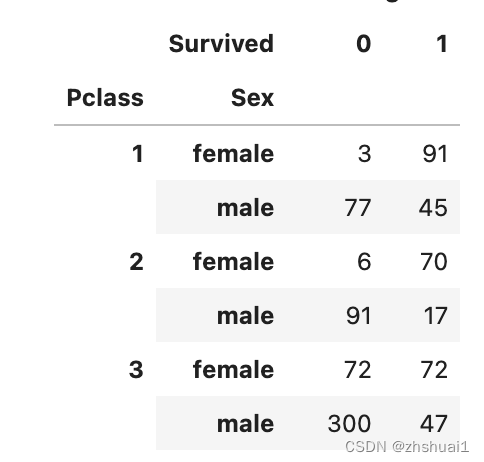
诚然，划分更详细，但总结后发现，仅以性别作为特征并不能提高准确率(或所有男性都死了，女性都活着)

df = pd.read_csv('models/titanic/train.csv')
df.loc[df.Age.isnull(),'Age'] = df.Age.mean()
df.Age = df['Age'] // 3 * 3
mapping = {'male':0,'female':1}
df['Sex']=df['Sex'].map(lambda r: mapping[r])
df.loc[df.Age.isnull(),'Age']=0
df = df[['Survived', 'Age','Pclass', 'Sex','SibSp','Fare']]
df.corr()

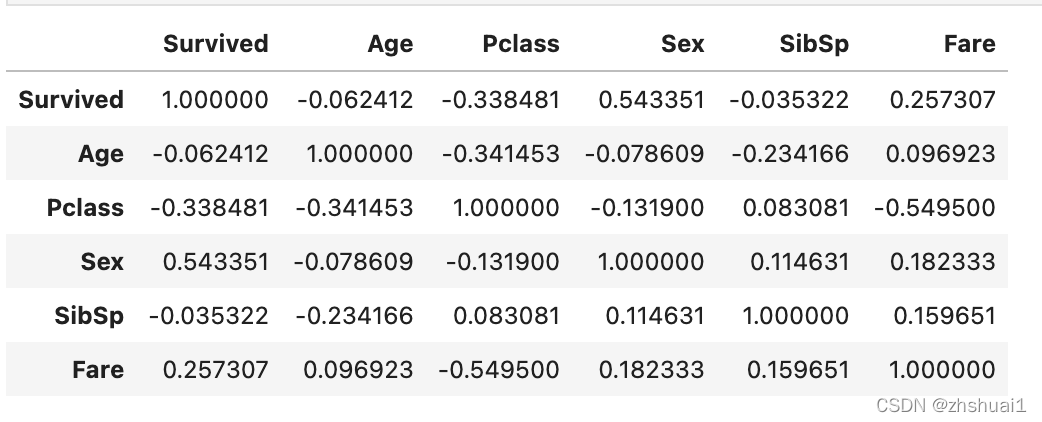
从这张图表还可以看出，相关性最大的数据是存活率和性别，以及门票和级别(0.5以上)，这更自然。

Original: https://blog.csdn.net/zhshuai1/article/details/121759428
Author: zhshuai1
Title: Titanic数据分析